During this post will explain about machine learning (ML) concepts i.e. Gradient Descent and Cost function. In logistic regression for binary classification, we can consider an example for a simple image classifier that takes images as input and predict the probability of them belonging to a specific category.
Let’s take an example of Gradient Descent and Cost function with a Cup image. We want to know the chance/probability of an image being a Cup.
Neural Network:
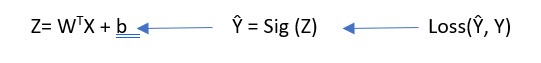
Let consider a very basic Neural network with just one neuron and layer. And, we want to know the probability Ŷ of it being a Cup (Y=1) for a given input image or feature set X.
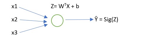
Ŷ can be consider as a linear function as Ŷ = WTX + b.
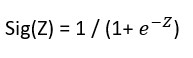
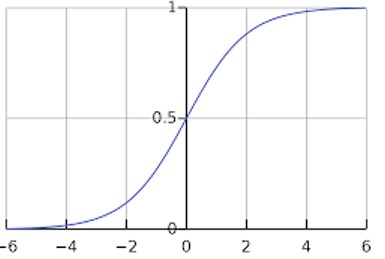
But this could be more than or less than one and we want to know the probability. We need to use a function like sigmoid which would give us the probability 0 ≤ Ŷ ≤ 1.
Ŷ = Sig(WTX + b) where Sig is called sigmoid function whose value lies between 0 and 1.
If horizontal axis in the value of Z then the sigmoid function’s value will lie between 0 and 1. Sig(Z), which plots on the vertical axis, is Zero for small values of Z and 1 for large values of Z.
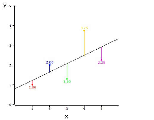
So basically, in Logistic regression, we aim to learn parameters W and b where b is the interceptor and W is the slope of the line, which best fit the line or which minimizes errors of prediction.
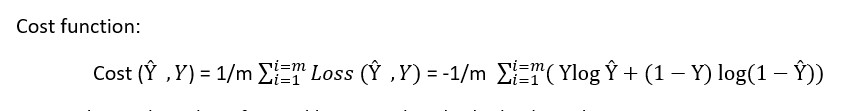
Error or loss function:
Error or loss function can be expressed in terms of the predicted value for a true label Y = 1/2 (Ŷ – Y)2 but this would be a non-convex function that would not give global optima, though it may have many local optima. So, in place of this, we can define the loss function as follows
Loss (Ŷ, Y) = – (Y log Ŷ + (1-Y) log (1- Ŷ) )
So, For true label of Y =1:
Loss (Ŷ, Y) = – Y log Ŷ and to make it as small as possible,
Ŷ should be large so the loss function will try to push the parameters W and b to make Ŷ as large.
For the true label of Y =0:
Loss = – log (1- Ŷ) and to make it as small as possible,
Ŷ should be as small as possible so the loss function will push the parameter W and b to make Ŷ smaller.
Loss function defines how well we do for a particular example, where cost function tells how well it does on the entire training set, so we aim to find the W and b which will minimize the overall Cost function
Cost funcNow to know the value of W and b we need to do the backward propagation
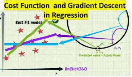
Now we can use Gradient descent to learn the parameters W and b for the entire training set. We want to find W and b which make minimize the Cost function .
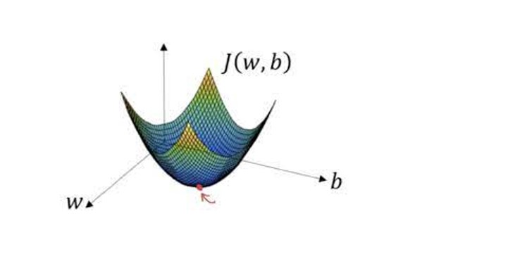
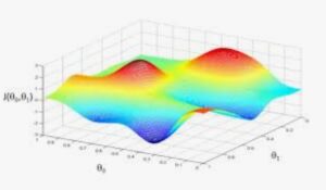
Convex Function:
As this function is convex, we can try to reach near about the global optima which are marked in red. We can initialize the value from any random number and through the iterations, we try to reach the point where the new values of W, b will
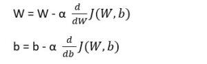
This implies that we want to take a step by changing the values of W and b based on the learning rate α. We can also considered how small or big a step we want to take and the slop of the step is given by
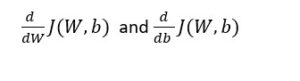
in W and b directions respectively.
To get deep dive into Technical details , Please Click here.